LeCun's World Models: JEPA, LeJEPA, LeWorldModel & H-JEPA
A technical walkthrough of the JEPA world-model line — the maths, a PyTorch reconstruction, H-JEPA's hierarchy, theory and planning results.
There are four distinct but tightly linked artifacts people lump together as "LeCun's world model":
- LeJEPA (Balestriero & LeCun, Nov 2025, arXiv 2511.08544) — the self-supervised representation learning theory + method.
- LeWorldModel / LeWM (Maes, Le Lidec, Scieur, LeCun, Balestriero, Mar 2026, arXiv 2603.19312) — the actual world model that puts LeJEPA's principle into an action-conditioned predictor trained from pixels.
- "When Does LeJEPA Learn a World Model?" (May 2026, arXiv 2605.26379) — the identifiability theory proving when the recovered latents are the true ones.
- H-JEPA (Zhang, Terver, Rabbat, LeCun & Balestriero, 5 October 2026, arXiv 2610.06805v1) — hierarchical prediction and planning across learned latent spaces.
These come out of LeCun's research circle around his post-Meta startup, AMI Labs (Advanced Machine Intelligence).
Why a world model, not an LLM
LeCun's thesis (from his 2022 position paper "A Path Towards Autonomous Machine Intelligence") is that intelligence requires an internal world model: a function that predicts how the world evolves, especially as a consequence of actions, so an agent can plan by simulating futures rather than reacting token-by-token.
The central design choice is where you predict:
- Generative models (LLMs, video diffusion, pixel-space world models) predict in observation space — the next token or frame in pixels. This wastes capacity on intrinsically unpredictable detail (every leaf, texture, sensor noise).
- JEPA (Joint Embedding Predictive Architecture) predicts in a learned latent space. Encode observations to abstract embeddings and predict the embedding of the future, discarding what is unpredictable.
That single move — predict in latent space, not pixel space — is the whole conceptual backbone.
JEPA & the collapse problem
Given two views of a signal (a context \(x\) and a target \(y\) — two crops, or observation-at-\(t\) and observation-at-\(t{+}1\)): an encoder \(f_\theta\) maps each to embeddings \(s_x = f_\theta(x)\), \(s_y = f_\theta(y)\); a predictor \(g_\phi\) predicts the target embedding from the context, optionally conditioned on an action \(a\): \(\hat s_y = g_\phi(s_x, a)\); and an energy measures incompatibility: \(E(x,y) = \lVert \hat s_y - s_y \rVert^2\).
JEPA / LeWorldModel data flow. The predictor models latent dynamics conditioned on the action; the prediction energy is computed entirely in embedding space, while SIGReg pulls the embedding distribution toward an isotropic Gaussian to prevent collapse.
This is an energy-based model: low energy = "these go together," and in the world-model case the predictor is the dynamics model. The fatal failure mode is collapse: if \(f_\theta\) maps everything to a constant, prediction loss is trivially 0 and the energy landscape is flat. Every JEPA's core engineering problem is preventing collapse while keeping a simple prediction loss.
| Method | Anti-collapse mechanism |
|---|---|
| SimCLR / contrastive | Negative samples push apart (needs huge batches) |
| BYOL / SimSiam | Stop-gradient + EMA "teacher" + predictor asymmetry |
| VICReg / Barlow Twins | Explicit variance + covariance penalties |
| I-JEPA (2023, images) | Masked prediction + EMA target encoder |
| V-JEPA / V-JEPA 2 (2024–25) | Masked spatiotemporal prediction, scaled to video |
| DINO-WM (2024) | Frozen pre-trained DINO features as the latent space |
LeJEPA and LeWM replace several stabilization heuristics with a principled regularizer, SIGReg. H-JEPA qualifies this story: a non-collapsed embedding distribution can still discard the agent, requiring an additional action-sensitive objective on diverse scenes (see below).
LeJEPA: making it provable
Key theoretical claim: the isotropic Gaussian is the unique embedding distribution that minimizes worst-case downstream prediction risk. If you don't know the downstream task, the optimal thing your embeddings can do is be distributed as \(\mathcal N(0, I)\) — maximally spread, no privileged directions, no collapse.
So instead of ad hoc variance/covariance terms, you directly regularize toward isotropic Gaussian via SIGReg (Sketched Isotropic Gaussian Regularization): draw random unit directions and project embeddings onto each (a distribution is isotropic Gaussian iff every 1-D projection is standard Gaussian — Cramér–Wold); then test each projection against \(\mathcal N(0,1)\) with a characteristic-function goodness-of-fit statistic (Epps–Pulley):
This is linear \(O(N)\) in time/memory — no negatives, no teacher, no stop-gradient, no EMA. The total objective has essentially one hyperparameter:
A faithful PyTorch reconstruction of SIGReg (illustrative, not copied from the official repo):
import torch

def epps_pulley_1d(p, ts, weight):
    # p: (N,) standardized projections; compare ECF to N(0,1) CF
    tp = ts[:, None] * p[None, :]                 # (T, N)
    re = torch.cos(tp).mean(dim=1)                # Re phi_hat(t)
    im = torch.sin(tp).mean(dim=1)                # Im phi_hat(t)
    target = torch.exp(-0.5 * ts**2)              # CF of N(0,1)
    diff2 = (re - target)**2 + im**2              # |phi_hat - phi_gauss|^2
    return (diff2 * weight).sum()

def sigreg(Z, n_dirs=256, n_freq=64, t_max=5.0):
    N, D = Z.shape
    Z = (Z - Z.mean(0)) / (Z.std(0) + 1e-6)       # center / scale per dim
    U = torch.randn(D, n_dirs, device=Z.device)
    U = U / U.norm(dim=0, keepdim=True)           # random unit directions
    P = Z @ U                                      # sketched 1-D projections
    P = (P - P.mean(0)) / (P.std(0) + 1e-6)
    ts = torch.linspace(0.05, t_max, n_freq, device=Z.device)
    w = torch.exp(-0.5 * ts**2)                    # Gaussian frequency weighting
    return torch.stack([epps_pulley_1d(P[:, k], ts, w) for k in range(n_dirs)]).mean()
LeWorldModel — the actual world model
Authors: Lucas Maes, Quentin Le Lidec, Damien Scieur, Yann LeCun, Randall Balestriero (Mila / NYU / Samsung SAIL / Brown). It is the first JEPA world model that trains stably end-to-end from raw pixels with only two loss terms — applying the LeJEPA insight to action-conditioned dynamics.
- Encoder \(z_t = \mathrm{enc}(o_t)\) — maps a pixel frame to a single ~192-dim token (≈200× fewer than DINO-WM's patch tokens).
- Predictor \(\hat z_{t+1} = \mathrm{pred}(z_t, a_t)\) — latent dynamics conditioned on action \(a_t\).
- ~15M parameters, trainable on a single GPU in a few hours.
This drops the hyperparameter count from six to one vs. the only prior end-to-end JEPA world model. Empirically it plans up to 48× faster than foundation-model-based world models, stays competitive on diverse 2D/3D control, encodes real physical structure (probeable), and reliably spikes its prediction error on physically implausible events ("surprise").
What makes it a world model rather than just an encoder: roll the predictor forward over candidate action sequences and pick the one whose imagined latent trajectory reaches the goal (CEM-style MPC, entirely in latent space):
@torch.no_grad()
def plan_mpc(enc, pred, o_now, z_goal, action_dim, horizon=10,
             n_samples=512, iters=4, elite=64):
    z = enc(o_now)                                       # (1, d)
    mu  = torch.zeros(horizon, action_dim)
    std = torch.ones(horizon, action_dim)
    for _ in range(iters):
        A = mu + std * torch.randn(n_samples, horizon, action_dim)
        zt = z.expand(n_samples, -1).clone()
        cost = torch.zeros(n_samples)
        for h in range(horizon):
            zt = pred(zt, A[:, h])                       # imagine next latent
            cost += ((zt - z_goal)**2).sum(-1)           # distance-to-goal in latent
        idx = cost.topk(elite, largest=False).indices    # keep best action seqs
        mu, std = A[idx].mean(0), A[idx].std(0) + 1e-4    # refit sampling dist
    return mu[0]                                          # execute first action, replan
Same family as PlaNet / Dreamer MPC-over-imagination, but the dynamics live in a non-generative, SIGReg-regularized latent rather than a reconstructive RSSM.
When does it learn a world model?
The theory paper (arXiv 2605.26379) answers when the recovered latents are the true hidden variables (identifiability):
- Theorem 5.1 (Linear Identifiability). Under a Gaussian world model, LeJEPA recovers the true latents up to an orthogonal rotation \(Q\); the alignment loss obeys \(\mathcal L(h) \ge 2(1-\rho)n\), with equality iff \(h(z) = Qz\).
- Theorem 5.2 (Gaussian Uniqueness). The Gaussian is the unique latent distribution (in the class) giving linear identifiability — the converse that justifies SIGReg's target.
- Theorem 5.3 (Graceful degradation). Approximate recovery with error \(\sim \delta / (2\rho(1-\rho))\) + regularization error.
Assumptions: independent latent components/transitions, stationarity, and additive Ornstein–Uhlenbeck noise \(z' = \rho z + \sqrt{1-\rho^2}\,\eta\). For Gaussian latents the transition operator's eigenfunctions are Hermite polynomials with eigenvalues \(\rho^d\), so any nonlinear map strictly reduces cross-correlation.
Honest limitation: the guarantees hold under Gaussian latents + OU dynamics + good exploration, and only for the encoder — not the action-conditioned predictor. So "LeWM provably learns the true world model" is not yet established; the dynamics side remains empirical.
H-JEPA: a hierarchy for long-horizon planning
October 2026 update. H-JEPA: End-to-End Learning of Hierarchical World Models for Visual Planning, by Wancong Zhang, Basile Terver, Michael Rabbat, Yann LeCun and Randall Balestriero, extends LeWM beyond a single prediction timescale.
Summary: predict and plan at different scales
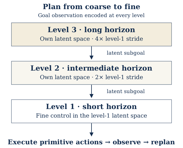
Each level learns its own latent space, action encoder and predictor; upper objectives backpropagate through lower encoders. Longer horizons can discard leg-pose detail while retaining maze position. This selective abstraction depends on separated timescales; manipulation datasets show less of it. Planning descends from goal to latent subgoals to primitive actions. Lower planners compare predictions with subgoals in the upper latent space. See the authors' method overview.
Main theoretical contributions
Appendix L formalizes slow-feature collapse:
- Proposition 1: with a readable, episode-constant background having an atomless distribution, an encoder can satisfy a marginal regularizer while ignoring motion; an identity predictor achieves zero prediction error.
- Theorem 1: optimal squared prediction error is bounded below by innovation variance. Zero error requires embeddings to evolve deterministically given their current state and action. Background-only codes qualify; the theorem does not select useful features among zero-loss solutions.
- Proposition 3: collapsed codes incur inverse-dynamics error at least equal to residual action variance given background, normalized by action dimension. It equals one for unit-variance actions unpredictable from background.
Thus SIGReg can preserve distributional diversity without preserving control information. Inverse dynamics predicts actions from consecutive latents, adding a temporal constraint; it does not guarantee distractor removal or physical-robot success. The timescale-abstraction findings are empirical, not universal identifiability guarantees.
Practical results
| Evaluation | Reported result |
|---|---|
| Visual AntMaze | Flat LeWM: 18.0%; three-level H-JEPA: 73.3% success (+55.3 percentage points). |
| FourRoom, AntMaze, Cube | Up to three levels improve the success–planner-compute frontier. |
| Push-T | Two levels help; deeper hierarchies deteriorate, plausibly because short episodes reduce usable training data. |
| DROID videos | 33.57 ± 1.52% fidelity for LeWM + inverse dynamics; 38.42 ± 0.94% for two-level H-JEPA. The compute sweep also favors hierarchy. |
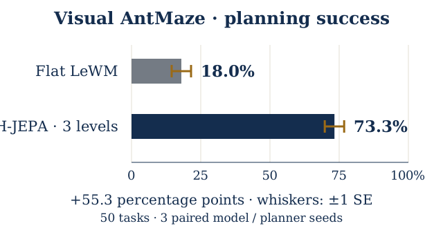
AntMaze uses 50 start–goal tasks; figures aggregate three paired training/planner seeds. Sources: official evaluation protocol and results, authors' results overview.
Ablations separate abstract goal costs from temporal decomposition: projecting a flat rollout into an upper latent can help on its own; subgoal planning adds another benefit. DROID measures Fréchet fidelity of end-effector paths, not closed-loop task success: stationary is 0%, expert is 100%. Frozen-encoder references use 1 fps versus H-JEPA's 5 fps, limiting direct comparison. See the project's DROID discussion.
Trying it
The official repository releases training, planning, probes and reproduction scripts, plus checkpoints. After installation and dataset/task preparation, run from h_jepa/:
python main_hjepa.py --config-name ant_hjepa_l3 seed=42
Training includes planning evaluation. Downloaded checkpoints allow evaluation without retraining; DROID evaluation needs only the released clips and models. These are the authors' results, not experiments reproduced for this post.
Relation to other work
Direct ancestry (LeCun's own line): I-JEPA → V-JEPA / V-JEPA 2 → LeJEPA → LeWorldModel → H-JEPA — from representation regularization to action-conditioned dynamics and hierarchical planning.
| Work | Relation |
|---|---|
| Ha & Schmidhuber, "World Models" (2018) | VAE + MDN-RNN dynamics + controller. The original; generative latent. |
| PlaNet / Dreamer v1–v3 | RSSM latent dynamics with a reconstruction loss. LeWM shares latent-MPC but drops reconstruction. |
| DINO-WM (2024) | Closest baseline; uses frozen DINO features. LeWM trains the encoder end-to-end with a ~200× smaller token. |
| Genie / Genie 2, Sora-as-world-model | Generative, pixel-space — exactly what LeCun argues against. |
| Causal-JEPA, Var-JEPA, Rectified Lp-JEPA (2026) | Community spinoffs extending JEPA + distributional regularizer. |
The unifying contrast: predict-in-latent + distributional regularizer (LeCun camp) vs. predict-in-observation-space / generative (LLM + video-diffusion camp).
The AMI startup
AMI Labs (Advanced Machine Intelligence), founded by LeCun after leaving Meta, raised a ~$1.03B seed round (announced ~March 2026) — among the largest AI seed rounds ever, on an explicit thesis: build world models, a contrarian bet against LLMs as the path to human-level intelligence. Critical coverage stresses that the funding-round framing oversells novelty — the theory only guarantees encoder-side recovery under idealized assumptions, and the world-model dynamics side remains empirical.